Linear Quadratic EstimationEven though modeling reality is mostly difficult in life, approximation is possible via predictions which is updated by observations. Initial predictions which do not depend on well analogical inferences, may cause high deviations. But, these predictions may be better if their effects are measurable, follow certain patterns and the results are evaluated, properly. Deviation from reality, may become lower with the inclusion of experience.
Classical physics which looks deterministic, deviates from reality because of factors which are not considered in equation. So, predictions should be revised to avoid from increasing deviation. Equations are just models and they are not equivalent to reality. Results differ slightly from actual. But, small errors increase with the time and deviation increases.
 For example, the measurements made with inertial measurement unit (IMU) of an unmanned aerial vehicle (UAV), have small errors because of limited accuracy. These small errors grow and mislead the UAV. So, Linear Quadratic Estimation (Kalman filter) is used for improving predictions.
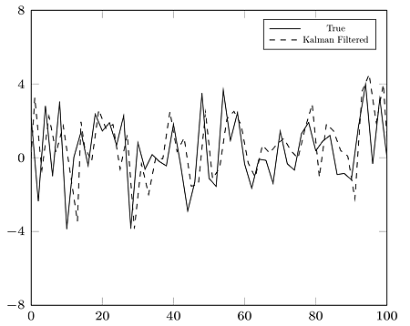
Although Kalman filter is called as a filter, it is used for a prediction tool in various fields. Literally, it filters the noise and based on prediction, comparison, update and revised estimation stages.
For example, the measurements made with inertial measurement unit (IMU) of an unmanned aerial vehicle (UAV), have small errors because of limited accuracy. These small errors grow and mislead the UAV. So, Linear Quadratic Estimation (Kalman filter) is used for improving predictions.
Although Kalman filter is called as a filter, it is used for a prediction tool in various fields. Literally, it filters the noise and based on prediction, comparison, update and revised estimation stages.
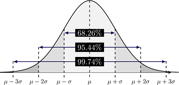
 Statistics comes into play here. In a non-deterministic, stochastic systems, it’s not possible to get 100% accurate results because of system noise and measurement noise. If the system is linear and the noise is Gaussian, Kalman filter’s approximation is better. "Gaussian", also known as “Normal distribution” is seen in this condition. Weighted average variance is calculated and when it decreases, precision increases.
 For the constant
  , at first, the estimated value is , at first, the estimated value is  with with  variance at variance at  . .
 And, the estimated value is
  with with  variance at variance at  .
The weighted average of these, .
The weighted average of these,


 The new entries made in the following manner,
 And the variance is updated.
 As you see, these operations can be done, recursively.
Estimation is done before the observation at
As you see, these operations can be done, recursively.
Estimation is done before the observation at  again. again.
 And correction is done depending on observation.
 Kalman filter works in this way as a dynamic model.
Kalman gain is "weight" depending on
Kalman filter works in this way as a dynamic model.
Kalman gain is "weight" depending on  and and  .
These formulas are seen when we look at Kalman filter, .
These formulas are seen when we look at Kalman filter,
 At first, k is index of discrete time.
  is estimation value and is estimation value and  is previous estimation value, is previous estimation value,  is control value and is control value and  is previous noise value.
A; state transition matrix, B; control matrix, H; observation matrix. is previous noise value.
A; state transition matrix, B; control matrix, H; observation matrix.
 is measured value, is measured value,  is measurement noise.
These formulas are used in estimation period, is measurement noise.
These formulas are used in estimation period,

 , estimation value at k, , estimation value at k,  is value (before the measurement, after the estimation). is value (before the measurement, after the estimation).  is co-variance (before measurement), Q is estimated error co-variance.
In the measurement update stage, these formulas are seen, is co-variance (before measurement), Q is estimated error co-variance.
In the measurement update stage, these formulas are seen,
 Pre-fit residual is calculated with this formula,
 And then Kalman gain is calculated,
 (R is measurement error co-variance)
With
(R is measurement error co-variance)
With  co-variance is updated.
Summary,
1. Estimation before the measurement. co-variance is updated.
Summary,
1. Estimation before the measurement.
 2. Estimation of the error co-variance.
 3. Kalman gain is calculated.
4. Estimation update stage
5. Error co-variance is updated.
There is also an extended version of the Kalman filter for nonlinear systems. It is transforming nonlinear to linear by using Jacobian matrices. Generally, the Kalman filter formulas are the same after the initial steps.
3. Kalman gain is calculated.
4. Estimation update stage
5. Error co-variance is updated.
There is also an extended version of the Kalman filter for nonlinear systems. It is transforming nonlinear to linear by using Jacobian matrices. Generally, the Kalman filter formulas are the same after the initial steps. |